Inference: find.saddlepoint.MLE()

find.saddlepoint.MLE() is the main high-level function for maximum-likelihood estimation (MLE) under a saddlepoint approximation (SPA).
compute.spa.negll() is the corresponding low-level tool for evaluating the saddlepoint negative log-likelihood (and, optionally, its derivatives).

What `find.saddlepoint.MLE()` returns

At a minimum, the output contains:

MLEs.theta: the fitted parameters $\hat\theta$ ,
MLEs.tvec: the fitted saddlepoint solution $\hat t$ (same length as the data),
std.error when std.error = TRUE,
discrepancy when discrepancy = TRUE, etc.

The two optimisation strategies

find.saddlepoint.MLE() supports two fitting options:

method = "constrained" (default): Joint optimisation over (tvec, theta) using nloptr, while enforcing the saddlepoint equation $K'(t;\theta) = y$ as equality constraints. This is robust and is the recommended default, especially when the CGF has a non-trivial domain constraint on tvec via cgf$ineq_constraint(tvec, theta).
method = "two_step": optimizes over $\theta$ only; for each $\theta$ it computes the saddlepoint solution $\hat{t}(\theta)$ internally (analytic if available, otherwise numerical solvers (Newton, or via constrained solvers)). This keeps the outer optimization low-dimensional and can be easier to tune. However, method = "two_step" is optimized for cases where the saddlepoint equation can be solved efficiently for each candidate $\theta$ (e.g., via an analytic $\hat t(\theta)$ or an unconstrained tvec path).

In the current implementation, if the CGF imposes a non-trivial domain/inequality constraint on tvec via cgf$ineq_constraint(tvec, theta) and no analytic $\hat t(\theta)$ is available, can be much slower. In such cases we recommend the default method = "constrained". Future versions may improve performance for constrained CGFs under method = "two_step".

Practical recommendation

Use method = "constrained" when:
- the CGF has a non-trivial domain constraint on tvec, or
- you want the most robust default behaviour.
Use method = "two_step" when:
- tvec is unconstrained (or an analytic $\hat t(\theta)$ exists)

Other arguments

Model parameters:
- starting.theta, lb.theta, ub.theta control the outer optimisation in $\theta$ .
Saddlepoint variable (usually you can leave these alone):
- starting.tvec, lb.tvec, ub.tvec can help if you need to guide the saddlepoint solver or enforce bounds.
Approximation flavor:
- zeroth.order = TRUE uses the zeroth-order SPA objective (no first-order correction term).
Extras:
- std.error = TRUE computes standard errors.
- discrepancy = TRUE computes the package’s discrepancy diagnostic/approximation.

Example 1: Gamma model (both methods)

Here we fit Gamma parameters (shape/rate) using the saddlepoint likelihood.


set.seed(1)
n <- 40
alpha_true <- 8
beta_true  <- 2
x <- rgamma(n, shape = alpha_true, rate = beta_true)

# constrained (joint over tvec and theta) 
res_con <- find.saddlepoint.MLE(
  observed.data   = x,
  cgf             = GammaCGF,
  starting.theta  = c(alpha = 5, beta = 1),
  lb.theta        = c(1e-6, 1e-6),
  ub.theta        = c(Inf, Inf),
  method          = "constrained",
  std.error       = TRUE,
  discrepancy     = TRUE
)

# two-step 
res_two <- find.saddlepoint.MLE(
  observed.data   = x,
  cgf             = GammaCGF,
  starting.theta  = c(alpha = 5, beta = 1),
  lb.theta        = c(1e-6, 1e-6),
  ub.theta        = c(Inf, Inf),
  method          = "two_step",
  std.error       = TRUE,
  discrepancy     = TRUE
)

cbind(
  true        = c(alpha_true, beta_true),
  two_step    = res_two$MLEs.theta,
  constrained = res_con$MLEs.theta
)
#>      true  two_step constrained
#> [1,]    8 10.579017   10.579020
#> [2,]    2  2.758294    2.758295

res_two$std.error
#> [1] 2.3655400 0.6311805
res_two$discrepancy
#> [1] 0.16666667 0.04345543

Example 2: Aggregated successes from a random number of sessions

This example illustrates a compositional model where the exact likelihood can be awkward.

Sessions per day: $N \sim \text{Poisson}(\lambda)$
Successes per session: $X_i \sim \text{Binomial}(m, p)$
Observed daily total: $Y = \sum_{i=1}^N X_i$

We build the CGF of $Y$ compositionally, then fit $p$ .


set.seed(1)

B <- 40         # number of days
lambda <- 10    # mean sessions/day (fixed here)
m <- 20         # opportunities per session
p_true <- 0.08

# Latent sessions/day
N <- rpois(B, lambda)
# Observed daily totals
Y <- rbinom(B, size = N * m, prob = p_true)

# CGF blocks: N ~ Poisson(lambda), X ~ Binomial(m,p)
count_cgf <- PoissonModelCGF(
  lambda  = adaptor(fixed_param = lambda),
  iidReps = 1
)

summand_cgf <- BinomialModelCGF(
  n       = adaptor(fixed_param = m),
  p       = adaptor(indices = 1),
  iidReps = 1
)

# Randomly-stopped sum across B i.i.d. days
cgf_Y <- randomlyStoppedSumCGF(
  count_cgf   = count_cgf,
  summand_cgf = summand_cgf,
  # iidReps = B,
  block_size = 1
)

# ## OR
# Y <- as.numeric(cgf_Y$rsim(n = B, vector_length = 1, parameter_vector = p_true))

fit_p <- find.saddlepoint.MLE(
  observed.data  = Y,
  cgf            = cgf_Y,
  starting.theta = 0.05,
  lb.theta       = 1e-6,
  ub.theta       = 1 - 1e-6,
  method         = "two_step",
  std.error      = TRUE
)

c(p_true = p_true, p_hat_spa = fit_p$MLEs.theta)
#>     p_true  p_hat_spa 
#> 0.08000000 0.08048538
fit_p$std.error
#> [1] 0.005020156

Additional theta-only inequality constraints (non-box constraints)

Most constraints can be handled using lb.theta / ub.theta.
user.ineq.constraint.function() is intended for constraints that cannot be expressed as independent bounds.

Imagine you track daily event counts for three ordered risk groups (low / medium / high) over B days.

Let the per-day rates be $\theta = \left( \lambda_{\text{low}},\lambda_{\text{med}},\lambda_{\text{high}} \right),$ and suppose domain knowledge suggests a monotone trend: $\lambda_{\text{low}} \le \lambda_{\text{med}} \le \lambda_{\text{high}}.$

These may be enforced via custom reparameterization, but user.ineq.constraint.function() lets you state them directly while keeping the natural parameters.

This is strictly a toy example to illustrate how to use user.ineq.constraint.function().


set.seed(1)
B <- 30  

# Toy truth that violates monotonicity (to make the constraint bind obvious)
theta_true <- c(lambda_low = 3.0, lambda_med = 7.0, lambda_high = 5.0)

# Daily counts per group (3 by B); each column is a day
Y_daily <- rbind(
  low    = rpois(B, lambda = theta_true["lambda_low"]),
  medium = rpois(B, lambda = theta_true["lambda_med"]),
  high   = rpois(B, lambda = theta_true["lambda_high"])
)

# Observed totals over B days per group (length 3)
y <- rowSums(Y_daily)

# actual MLE
theta_uncon <- as.numeric(y) / B


# Build the CGF for totals
cgf <- PoissonModelCGF(lambda = function(theta) B * theta)

# ## We could also use rsim()
#  set.seed(1)
#  y <- as.numeric(cgf$rsim(n = 1, vector_length = 3, parameter_vector = c(lambda_low = 3.0, lambda_med = 7.0, lambda_high = 5.0)))


# NLOPT convention: constraints(theta) <= 0 is feasible.
# lambda_low <= lambda_med <= lambda_high
user_ineq <- function(theta){
  constraints <- c(
    theta[1] - theta[2],  # low - med <= 0
    theta[2] - theta[3]   # med - high <= 0
  )
  jacobian <- rbind(
    c( 1, -1,  0),
    c( 0,  1, -1)
  )
  list(constraints = constraints, jacobian = jacobian)
}

fit <- find.saddlepoint.MLE(
  observed.data = as.numeric(y),
  cgf           = cgf,
  starting.theta = c(1,2,3),
  lb.theta       = rep(1e-10, 3),
  ub.theta       = rep(Inf,   3),
  method         = "two_step",
  user.ineq.constraint.function = user_ineq
)

fit$MLEs.theta
#> [1] 3.1 6.0 6.0

# Note:
# - If you OMIT user.ineq.constraint.function(), the fit reduces to the usual Poisson MLE:
#     theta_uncon = y / B
# - Because we simulated a violation (med > high), we should expect lambda_med == lambda_high.

Likelihood evaluation: `compute.spa.negll()`

compute.spa.negll() evaluates the SPA negative log-likelihood at a given parameter_vector.
It can also return derivatives (gradient, hessian) which is useful for debugging or plugging into custom optimisers.


set.seed(1)
theta0 <- c(mu = 0, sigma = 1)
y <- as.numeric(NormalCGF$rsim(n = 10, vector_length = 1, parameter_vector = theta0))


nll <- compute.spa.negll(
  parameter_vector = theta0,
  observed.data    = y,
  cgf              = NormalCGF,
  gradient         = TRUE,
  hessian          = TRUE,
  spa_method       = "standard",
  tvec_source      = "auto"
)

nll$vals
#> [1] 12.01869
nll$gradient
#> [1] -1.322028  4.341394
nll$hessian
#>           [,1]     [,2]
#> [1,] 10.000000 2.644056
#> [2,]  2.644056 6.975817

Repeated likelihood evaluation and tape creation

When you request derivatives (gradient = TRUE and/or hessian = TRUE), compute.spa.negll() will (internally) build an RTMB tape and then evaluate it at the supplied parameter_vector.

If you need to evaluate the same SPA objective many times (e.g., inside your own optimisation loop), it is more efficient to build the tape once and reuse it. The package currently uses an internal helper for this:

saddlepoint:::create_spa_taped_fun() (internal function; may change without notice)

A minimal pattern is:


taped_nll <- saddlepoint:::create_spa_taped_fun(
  param_vec     = theta0,
  observed.data = y,
  cgf           = NormalCGF,
  spa_method    = "negll_standard",
  tvec_source   = "auto",
  gradient      = TRUE,
  hessian       = FALSE
)

# Now reuse without re-taping:
taped_nll(theta0)$vals
taped_nll(c(mu = 0.5, sigma = 1.2))$vals

SPA vs true MLE in the random-sum Binomial example


set.seed(5)
B <- 40; lambda <- 10; m <- 20
p_true <- 0.08

count_cgf <- PoissonModelCGF(lambda  = adaptor(fixed_param = lambda) )
summand_cgf <- BinomialModelCGF(
  n = adaptor(fixed_param = m),
  p = adaptor(indices = 1)
)
cgf_Y <- randomlyStoppedSumCGF(
  count_cgf   = count_cgf,
  summand_cgf = summand_cgf,
  block_size = 1
)
Y <- as.numeric(cgf_Y$rsim(n = B, vector_length = 1, parameter_vector = p_true))



# Exact likelihood 
.log_sum_exp <- function(v) {
  mx <- max(v)
  mx + log(sum(exp(v - mx)))
}
.log_pmf_compound_pois_binom <- function(y, p, lambda, m, n_max) {
  if (!is.finite(p) || p <= 0 || p >= 1) return(-Inf)
  n_min <- if (y == 0) 0L else as.integer(ceiling(y / m))
  n <- n_min:n_max
  log_terms <- dpois(n, lambda = lambda, log = TRUE) +
    dbinom(y, size = n * m, prob = p, log = TRUE)
  .log_sum_exp(log_terms)
}
.fit_exact_p <- function(Y, lambda, m) {
  n_max <- qpois(1 - 1e-12, lambda) + 80L
  nll <- function(p) {
    lp <- vapply(
      Y,
      function(yy) .log_pmf_compound_pois_binom(yy, p, lambda, m, n_max),
      numeric(1)
    )
    if (any(!is.finite(lp))) return(Inf)
    -sum(lp)
  }
  opt <- optimize(nll, interval = c(1e-6, 1 - 1e-6))
  list(p_hat = opt$minimum, nll = opt$objective, n_max = n_max)
}


# fit SPA 
fit_spa <- find.saddlepoint.MLE(
  observed.data  = Y,
  cgf            = cgf_Y,
  starting.theta = 0.05,
  lb.theta       = 1e-6,
  ub.theta       = 1 - 1e-6,
  method         = "two_step",
  std.error      = FALSE
)
p_spa <- as.numeric(fit_spa$MLEs.theta)

# fit exact
fit_ex <- .fit_exact_p(Y, lambda, m)
p_ex <- fit_ex$p_hat

# profile curves on a grid
p_grid <- seq(0.005, 0.25, length.out = 80)

# exact nll curve
nll_exact_grid <- vapply(p_grid, function(p) {
  .fit_exact_p(Y, lambda, m)$nll  # (simple but repeats work)
}, numeric(1))
n_max <- fit_ex$n_max
nll_exact_grid <- vapply(p_grid, function(p) {
  -sum(vapply(Y, function(yy) .log_pmf_compound_pois_binom(yy, p, lambda, m, n_max), numeric(1)))
}, numeric(1))


# SPA nll curve 
taped_nll <- saddlepoint:::create_spa_taped_fun(
  param_vec     = p_true,
  observed.data = Y,
  cgf           = cgf_Y,
  spa_method    = "negll_standard",
  tvec_source   = "auto",
  gradient      = FALSE
)
nll_spa_grid <- vapply(p_grid, function(p) { taped_nll(p)$vals}, numeric(1))


# Plot: profile curves - shifted 
y1 <- nll_exact_grid - min(nll_exact_grid, na.rm=TRUE)
y2 <- nll_spa_grid   - min(nll_spa_grid,   na.rm=TRUE)

plot(p_grid, y1, type="l", lwd=2, col="black",
     xlab="p", ylab="NLL - min(NLL)")
lines(p_grid, y2, lwd=2, lty=2, col="#2C7FB8")     
points(p_grid, y2, pch=16, cex=.5, col="#6A51A3")  

abline(v=p_true, lty=3, col="grey30")
abline(v=p_ex,   lty=1, col="black")
abline(v=p_spa,  lty=2, col="#2C7FB8")

legend("topright",
       legend=c("exact","spa","p_true","p_exact","p_spa"),
       col=c("black","#2C7FB8","grey30","black","#2C7FB8"),
       lty=c(1,2,3,1,2), lwd=c(2,2,1,1,1), bty="n")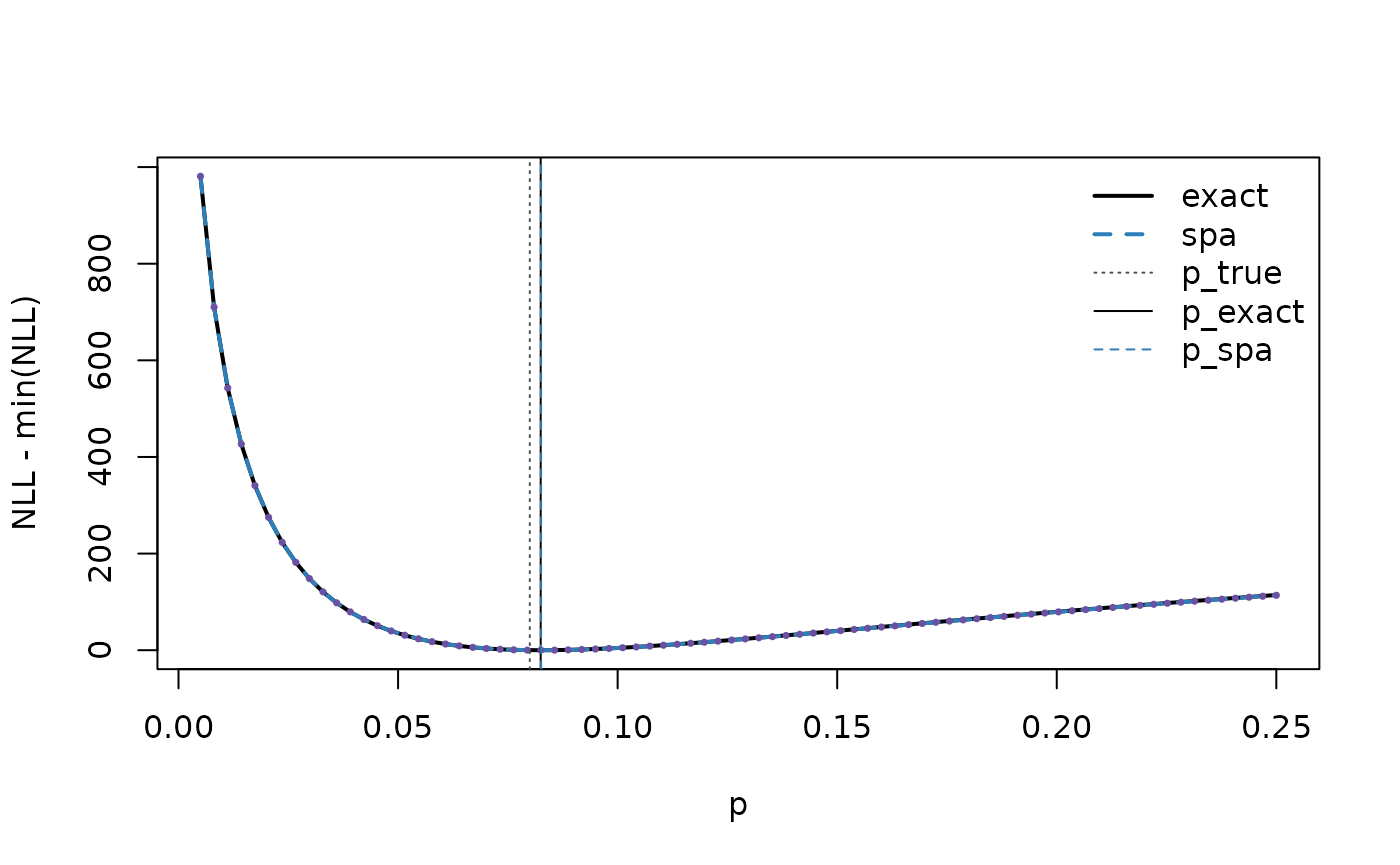

Exact and saddlepoint negative log-likelihood curves versus the parameter; minima indicate the two MLEs.

c(p_true = p_true, p_exact = p_ex, p_spa = p_spa)
#>     p_true    p_exact      p_spa 
#> 0.08000000 0.08247427 0.08256963

Control arguments

opts.user controls the nloptr optimiser (SLSQP). Common options include:
- maxeval, xtol_rel, ftol_abs, print_level
control.nlminb controls nlminb when method = "two_step" and no user.ineq.constraint.function is supplied. Common options include:
- eval.max, iter.max, rel.tol

What find.saddlepoint.MLE() returns